Piecing together scraps of causal inference intuition

I've been learning some basics of causal inference on and off. So far I've used two main references:

• Michael Nielsen's essay If correlation doesn’t imply causation, then what does?
• Judea Pearl and Dana Mackenzie's The Book of Why

These are interestingly complementary. Nielsen's essay is a detailed introduction to the mechanics of calculating with the do-calculus, from the perspective of someone actively working through the material to internalise it better.

For example, Nielsen discusses how to calculate the causal effect of smoking in this standard example that comes up in basically every introduction to the do-calculus:

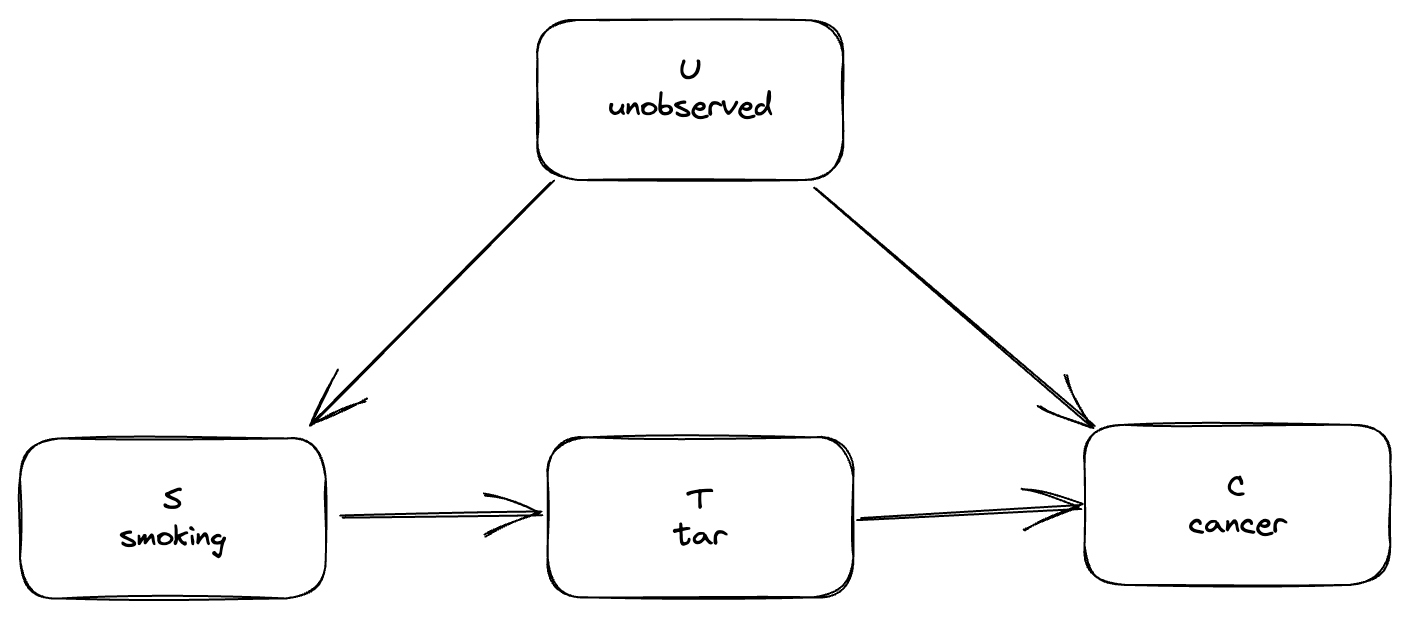
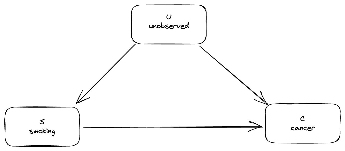
In this model, the effect of smoking (\(S\)) on cancer (\(C\)) is mediated by the presence of tar (\(T\)) in the lungs. There's also some unobserved factor \(U\) that affects both smoking and cancer (maybe a genetic propensity for both). It turns out that for this model you can calculate the causal effect of smoking on cancer in terms of observed probabilities, even in the presence of the unobserved factor. However, you can't do this in the following model without tar:

Nielsen works through the calculation for this by using the rules of the do-calculus, and the answer pops out at the end, but the process is not super enlightening. He's left with the following questions:

Something that bugs me about the derivation of equation [5] is that I don’t really know how to “see through” the calculations. Yes, it all works out in the end, and it’s easy enough to follow along. Yet that’s not the same as having a deep understanding. Too many basic questions remain unanswered: Why did we have to condition as we did in the calculation? Was there some other way we could have proceeded? What would have happeed if we’d conditioned on the value of the hidden variable? (This is not obviously the wrong thing to do: maybe the hidden variable would ultimately drop out of the calculation). Why is it possible to compute causal probabilities in this model, but not (as we shall see) in the model without tar? Ideally, a deeper understanding would make the answers to some or all of these questions much more obvious.

The Book of Why is sort of the opposite. It's a popular science book with lots of useful historical background and scraps of intuition, but almost no equations. This works pretty well for the early parts of the book, but by the time it gets on to more complicated things like the tar example the words-only explanations are extremely hard to follow.

Combining the two turns out to work well for propagating some understanding into the equations. I'm not the only person to notice this – the blog post Some "Causal Inference" intuition by Marcus Lewis uses the same sources – but I needed to spell out the details more for my understanding, so it seemed worth writing up.

What's so great about adding tar?

I'm going to focus on this question from Nielsen's list:

Why is it possible to compute causal probabilities in this model, but not (as we shall see) in the model without tar?

I find it easier to think about the problem if I put some actual numbers in, so I made some up. Note that I've just picked the numbers to be simple, different from each other so I make fewer stupid algebra mistakes, and sort of directionally correct. Other than that they are not supposed to be at all plausible!

First, here are my made-up probabilities of cancer (\(C=1\)) given all the options for presence or absence of smoking or tar:

$$\begin{eqnarray}p(C=1|S=0, T=0) &=& 0.1 \nonumber \\p(C=1|S=0, T=1) &=& 0.3 \nonumber \\p(C=1|S=1, T=0) &=& 0.6 \nonumber\ \\p(C=1|S=1, T=1) &=& 0.7 \nonumber \end{eqnarray}$$

Next, here are the probabilities of tar given smoking:

$$\begin{eqnarray}p(T=1|S=0)&=&0.2 \nonumber \\ p(T=1|S=1)&=&0.9 \nonumber\end{eqnarray}$$

Finally, let's say half of people in our made-up study smoke:

$$p(S=1) = 0.5$$

Now, we want to calculate \(p(C=1|\text{do}(S=1))\), the probability of getting cancer if we force someone to smoke, without actually forcing a whole lot of people to smoke and measuring the results. We can expand in terms of the tar variable:

$$p(C=1|\text{do}(S=1)) = \sum_{t=0,1} p(C=1|\text{do}(T=t))p(T=t|\text{do}(S=1)) $$

Think of this as saying that:

• either you end up with a tar state with \(p(T=1|\text{do}(S=1))\), in which case the likelihood of getting cancer is \(p(C=1|\text{do}(T=1))\)
• either you end up with a no-tar state with \(p(T=0|\text{do}(S=1))\), in which case the likelihood of getting cancer is \(p(C=1|\text{do}(T=0))\)

Now, what we're looking to do is get rid of the \(\text{do}\)s and write this out in terms of normal probabilities. To do this, we'll consider the paths between \(S\) and \(T\) and the paths between \(T\) and \(C\) one at a time.

Start with \(S\) to \(T\). There's one direct path, \(S\rightarrow T\), which is the causal path we're interested in. There's also an indirect path, \(S\leftarrow U\rightarrow C \leftarrow T\). However, that path is blocked by the collider at \(C\), so we can ignore it. The only unblocked path is the causal path, so we can drop the \(\text{do}\)s for this part:

$$p(T|\text{do}(S)) = p(T|S)$$

and the equation for \(p(C=1|\text{do}(S=1))\) above becomes

$$p(C=1|\text{do}(S=1)) = \sum_{t=0,1} p(C=1|\text{do}(T=t))p(T=t|S=1) $$

Now consider the path from \(T\) to \(C\). Again there's a direct path, \(T\rightarrow C\), and an indirect path, \(T \leftarrow S \leftarrow U \rightarrow C\). This time there's no collider, so we do have to take the indirect path into account. We can't do much about \(U\), because it's unobservable, but this doesn't matter because we can control for \(S\) instead:

$$p(C|\text{do}(T)) = \sum_{s=0,1} p(C|T,S=s)p(S=s)$$

We can stick this back into the equation for \(p(C=1|\text{do}(S=1))\) to get rid of the remaining \(\text{do}\):

$$p(C=1|\text{do}(S=1)) = \sum_{s=0,1}\sum_{t=0,1} p(C=1|T=t,S=s)p(S=s) p(T=t|S=1) $$

Now I'll plug my made-up numbers in:

$$\begin{eqnarray}p(C=1|\text{do}(S=1))  &=& p(C=1|T=0,S=0)\,p(S=0) \,p(T=t|S=1) \nonumber \\&+& p(C=1|T=0,S=1)\,p(S=1) \,p(T=t|S=1) \nonumber \\ &+& p(C=1|T=1,S=0)\,p(S=0) \,p(T=t|S=1) \nonumber\ \\ &+& p(C=1|T=1,S=1)\,p(S=1) \,p(T=t|S=1) \nonumber \end{eqnarray}$$

$$ \begin{eqnarray} &=& 0.1 \times 0.5 \times 0.1 \nonumber \\&+& 0.3 \times 0.5 \times 0.9 \nonumber \\ &+& 0.6 \times 0.5 \times 0.1 \nonumber\ \\ &+& 0.7 \times 0.5 \times 0.9 \nonumber \end{eqnarray}$$

$$=0.485$$

Similarly we can calculate what happens if we force someone to not smoke, to see exactly how bad smoking is in this model:

$$\begin{eqnarray}p(C=1|\text{do}(S=0))  &=& p(C=1|T=0,S=0)\,p(S=0) \,p(T=t|S=0) \nonumber \\&+& p(C=1|T=0,S=1)\,p(S=1) \,p(T=t|S=0) \nonumber \\ &+& p(C=1|T=1,S=0)\,p(S=0) \,p(T=t|S=0) \nonumber\ \\ &+& p(C=1|T=1,S=1)\,p(S=1) \,p(T=t|S=0) \nonumber \end{eqnarray}$$

$$ \begin{eqnarray} &=& 0.1 \times 0.5 \times 0.8  \nonumber \\&+& 0.3 \times 0.5 \times 0.2  \nonumber \\ &+& 0.6 \times 0.5 \times 0.8 \nonumber\ \\ &+& 0.7 \times 0.5 \times 0.2 \nonumber \end{eqnarray}$$

$$=0.38$$

So in this cruel world of my own invention, you have a 38% chance of getting cancer even if you don't smoke, but smoking does still have a considerable causal effect, increasing your chances to 48.5%.

Now let's quickly look at why this doesn't work in the model without tar. In the model without tar there are again two paths from \(S\) to \(C\): the direct causal path \(S\rightarrow C\) and the confounding path \(S\leftarrow U\rightarrow C\). This time there's nothing we can do about the confounding path: there's no collider to block it, and the only intermediate node of the path \(U\) is unobservable so we can't control for it. So we're out of luck.

Remaining questions

I definitely have a better understanding now of why the tar example works that's much more transparent than hitting the expression with the rules of the do-calculus several times until the answer pops out. I still wonder whether I can do even better and 'just see' intuitively why adding a noisy mediator like tar between the smoking and cancer nodes is so helpful.

It would also be nice to propagate some of this extra intuitive understanding back into the rules-based derivation. Maybe that will give me a better handle on why the rules of the do-calculus work.

Also, it would be good to analyse some other models that aren't this tar one that everyone uses all the time.